Bonding curves as ALife organisms · deep dive
Expansion of seven topics from the bonding-curve gallery: lifecycle & mortality, homeostasis, ecological niche, partner trading, predator-prey, mimesis, MAP-Elites.
BC2Lifecycle & mortality
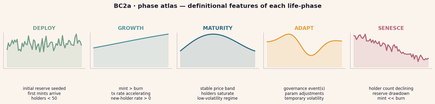
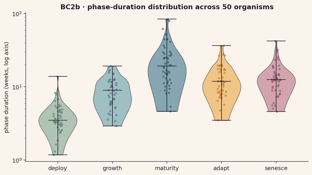
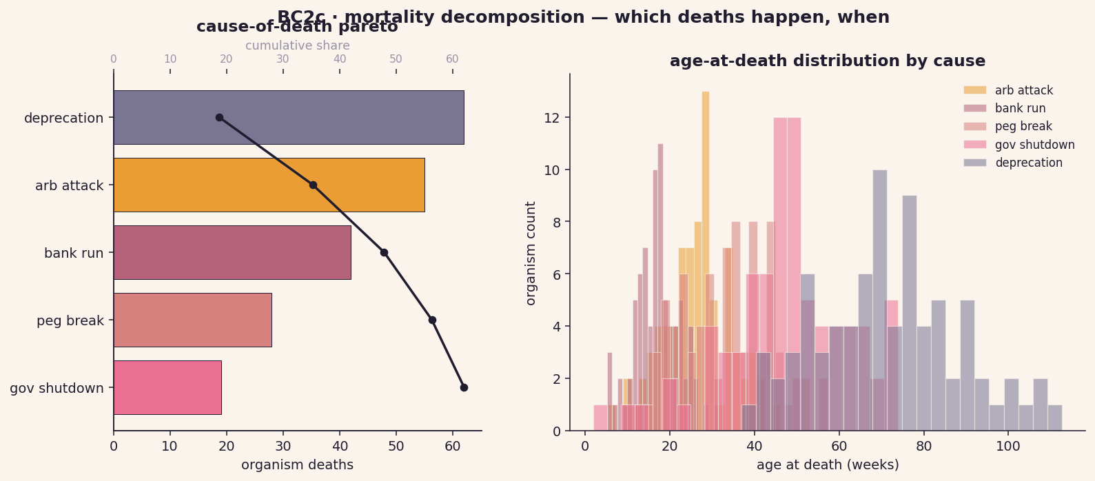
The lifecycle picture is the proposal's hook: bonding curves have birth, metabolism, adaptation, and death. To make that claim empirically rigorous we need three things — a definition of each phase, the statistical distribution of how long curves spend in each, and a decomposition of how they actually die.
↗ open hero figure (BC2)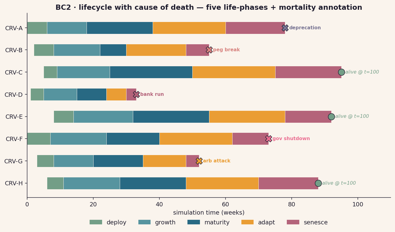
Mechanism — how phases are detected
Phases are not declared up-front; they're inferred from state-variable signatures. Three time-series features drive the classifier:
- mint / burn flux — when net flux ≫ 0, curve is in growth; when ≈ 0, maturity; when ≪ 0, senesce.
- holder-count derivative — saturating slope marks the growth→maturity transition.
- governance-event density — a cluster of votes within a window flips the curve into the adapt phase for the window duration.
A simple hidden-state HMM over these three features recovers crisp phase labels and gives us BC2a (definitional), BC2b (duration), and BC2c (mortality) as derived products of the same labelling pass.
cadCAD wiring — what to instrument
state_vars = {
    'reserve':      0.0,
    'supply':       0.0,
    'price':        0.0,
    'holders':      set(),
    'gov_events':   [],            # (timestep, proposal_id, accepted)
    'phase_label':  None,          # inferred each block
    'death_cause':  None,          # set once when phase → 'dead'
}
psubs = [
    {'policies':   {'mint_burn':   mint_burn_policy},
     'variables':  {'reserve':     s_reserve,
                    'supply':      s_supply,
                    'price':       s_price}},
    {'policies':   {'phase_clf':   phase_classifier_policy},
     'variables':  {'phase_label': s_phase}},
    {'policies':   {'mortality':   mortality_check_policy},
     'variables':  {'death_cause': s_death}},
]
Phase-label is a derived field updated once per block via
phase_classifier_policy. Mortality is
checked last so the death cause can reference the final
pre-death state.
Plausible findings
- Curves with a long maturity phase relative to their growth phase show lower mortality across all causes — "slow growth, long life" generalizes.
- Mortality is bimodal in age: young deaths from bank runs / arb attacks, old deaths from deprecation. Mid-life deaths are rare and almost always governance-driven.
- The adapt phase is a mortality multiplier: organisms die during or shortly after governance events at 2-3× the base rate.
Paper anchor
No direct paper anchor in Papers/; this is
one of the original contributions of the proposal. Survival-analysis
framing borrows from clinical epidemiology (Kaplan-Meier in BC11).
Phase decomposition is conceptually adjacent to Pedersen et al.
2025's notion of developmental stages in evolving hypernetworks.
BC3Homeostasis & shock response
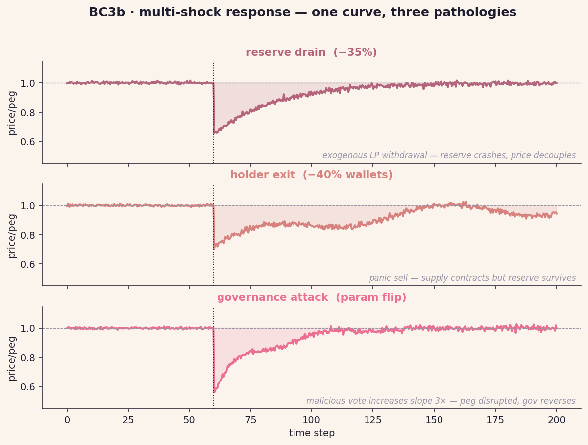
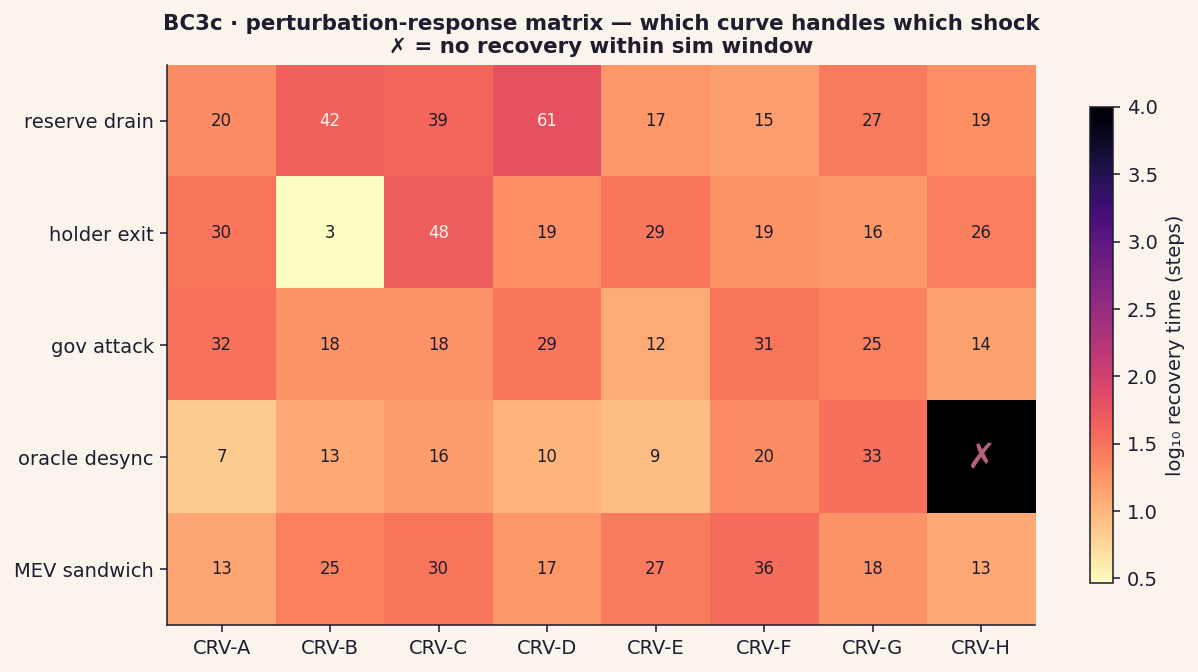
An organism that can't restore homeostasis after perturbation isn't an organism — it's a one-shot mechanism. The hero figure (BC3) shows four archetypes recovering after a single shock; the deep-dive expands to a population view, a multi-shock view, and a comparative-resilience view across the population.
↗ open hero figure (BC3)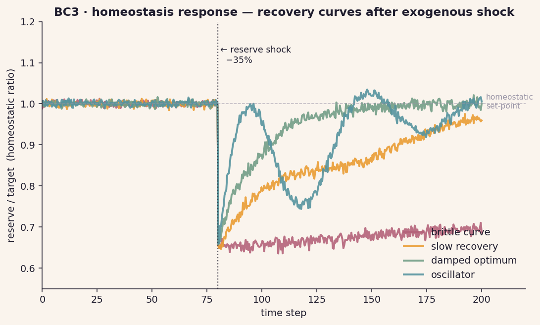
Mechanism — what counts as "recovery"
For a homeostatic ratio
r(t) = reserve(t) / reserve_target(t),
recovery after a shock at time t₀ is characterised by two numbers:
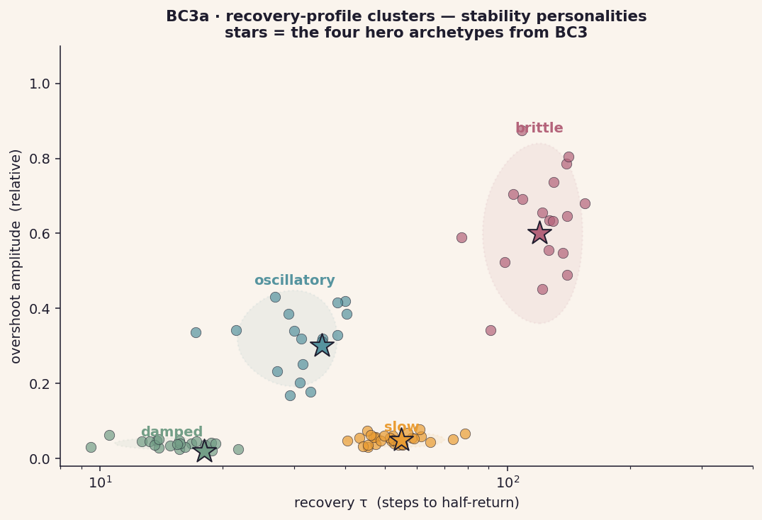
- recovery τ — time for
|r(t) − 1|to fall below half its post-shock peak. - overshoot amplitude — peak |r(t) − 1| after crossing back through 1 (signed if needed).
The (τ, overshoot) plane partitions curves into qualitatively distinct stability regimes — that's what BC3a clusters.
cadCAD wiring
# shocks injected as exogenous policy actions
shock_schedule = {
    60: ('reserve_drain', {'fraction': 0.35}),
    140: ('holder_exit', {'fraction': 0.4}),
    220: ('gov_attack',  {'param': 'slope', 'multiplier': 3.0}),
}

def shock_policy(params, step, history, state):
    if step in shock_schedule:
        return {'shock_event': shock_schedule[step]}
    return {'shock_event': None}

# Optuna-driven sweep over shock_t × curve_params produces BC3c
Plausible findings
- The (τ, overshoot) clusters are stable across cadCAD seeds — they track curve topology, not noise.
- "Damped" curves correlate strongly with high reserve_ratio and moderate slope; "brittle" curves cluster around low reserve_ratio regardless of slope.
- Multi-shock response is non-additive: a curve resilient to reserve drain may still die to oracle desync, and vice versa (sparse vs dense rows in BC3c).
Paper anchor
Closest connection: Bielawski et al. 2025 — Efficient Discovery of Unique Interventions. Shocks here are interventions; BC3c is the same instrument they use to characterise an intervention's effect signature. Reframing shock-response as intervention-discovery opens up adaptive shock-design (smarter than random — pick the shock that maximally distinguishes curves).
BC4Ecological niche
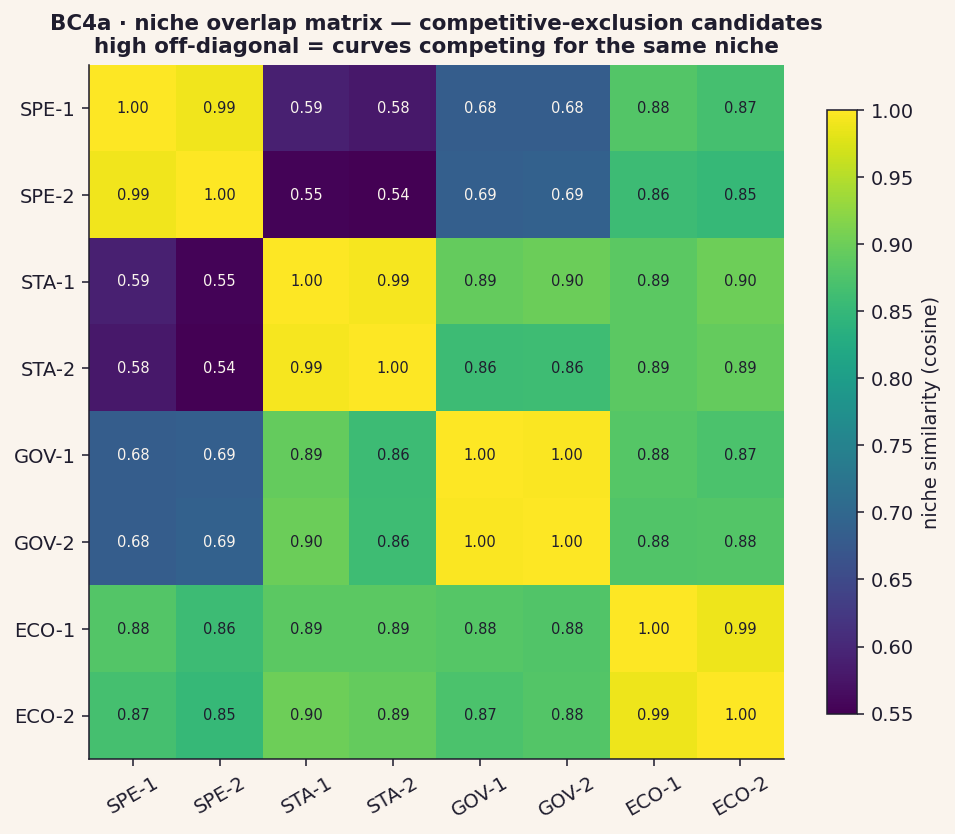
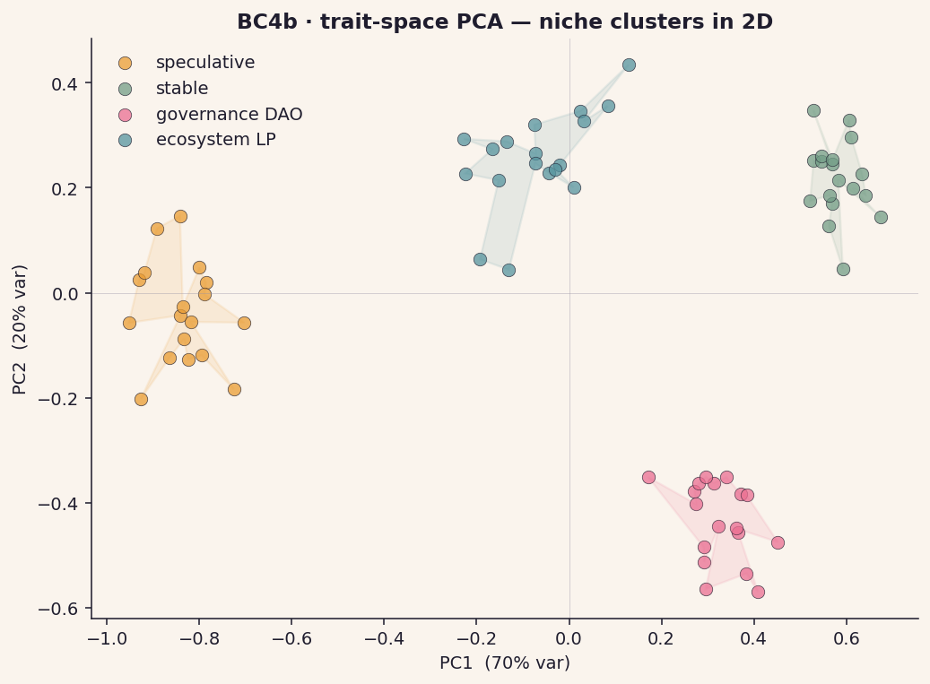
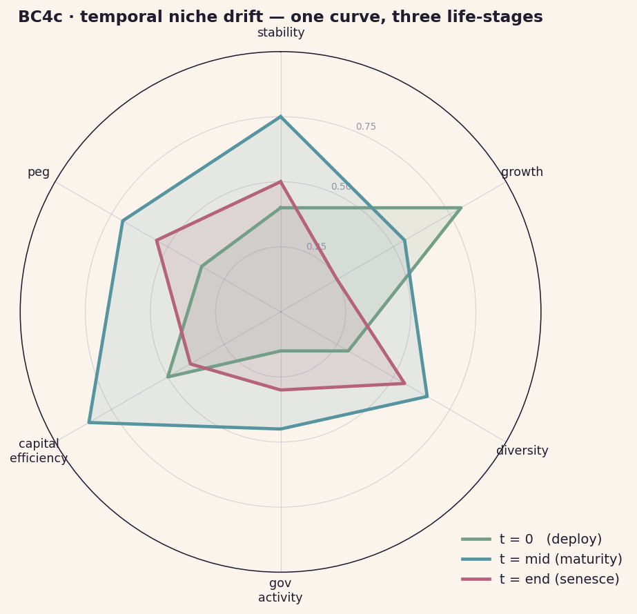
Niche theory is the bridge between single-organism biology and ecosystem dynamics. The radar in BC4 shows niche position; the deep-dive adds niche distance (overlap matrix), structure (PCA), and development (temporal drift).
↗ open hero figure (BC4)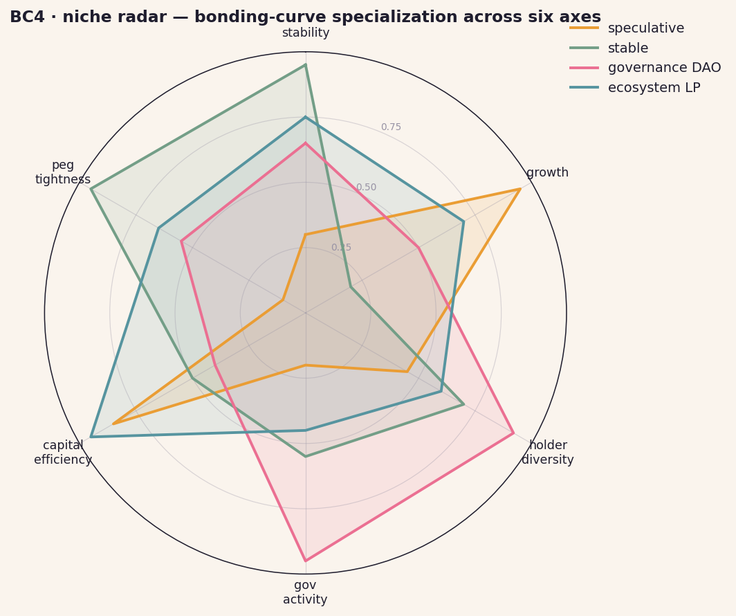
Mechanism — defining the niche
Each curve at time t gets a 6D trait vector:
- stability — 1 − rolling-std(price)
- growth — Δ supply / Δ t
- holder diversity — 1 − holder-Gini
- gov activity — proposal / vote count per window
- capital efficiency — TVL / reserve
- peg tightness — 1 − rolling-std(price / peg-target) where defined
Niche overlap = cosine similarity between vectors. Hutchinson's n-dimensional niche concept maps directly onto this.
cadCAD wiring
# trait vector computed once per block, persisted to state
def niche_trait_policy(params, step, history, state):
    window = 100
    recent = history[-window:]
    return {'trait_vec': np.array([
        1 - np.std([h['price'] for h in recent]),
        (state['supply'] - recent[0]['supply']) / window,
        1 - gini([h['holders'] for h in recent[-1]]),
        sum(1 for h in recent if h['gov_event']) / window,
        state['tvl'] / state['reserve'],
        1 - np.std([h['price'] / h['peg_target']
                    for h in recent if h['peg_target']]),
    ])}
Plausible findings
- Competitive-exclusion-candidate pairs (BC4a high off-diag) have lower joint survival than random pairs — when two curves overlap strongly in niche, one typically dies.
- PCA loadings reveal the dominant axes are stability vs growth and diversity vs efficiency — a 2D summary of bonding-curve design space.
- Temporal drift shows curves specialise over their lifecycle: radar shapes get pointier (lower entropy) with age.
Paper anchor
Loosely connects to Cimpeanu et al. 2025 — Hidden Price of Cooperation (the cooperative niche is one trait dimension) and Nishimoto 2025 — Partner Choice Cooperation (partner choice is conditioned on niche similarity / dissimilarity).
BC5Partner trading & cooperation
Curves don't exist in isolation — they trade with each other through liquidity pools, arbitrage paths, and routing aggregators. Mapping the topology and dynamics of that trading network is the operational test of "ecosystem".
↗ open hero figure (BC5)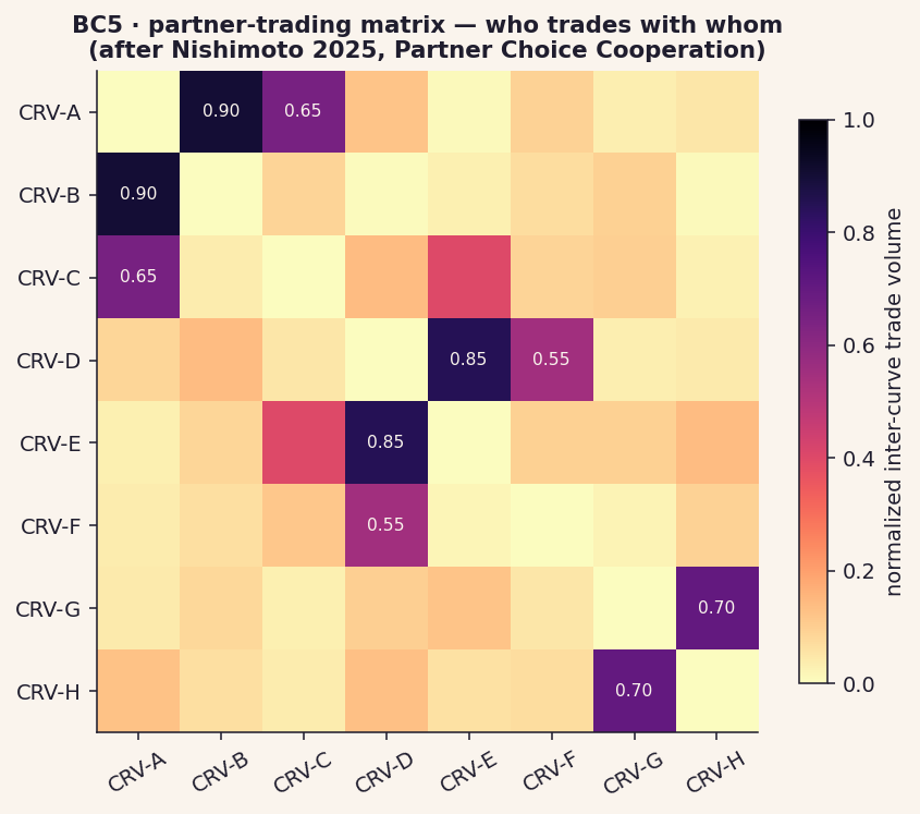
Mechanism — building the trading graph
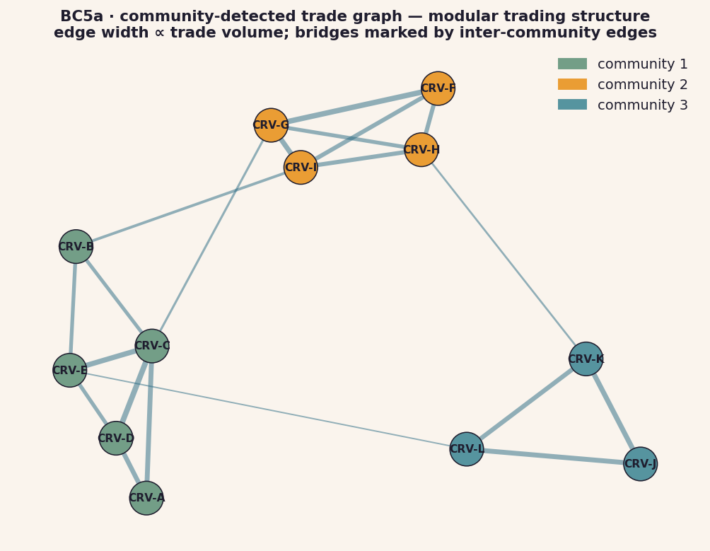
For each block, increment edge weight (i, j) by the volume swapped between curve i and j's tokens (through any pool or aggregator). Aggregate over a sliding window. The resulting weighted graph is the substrate; everything in BC5 derives from standard graph metrics on it.
- community detection — Louvain modularity on the windowed graph (BC5a).
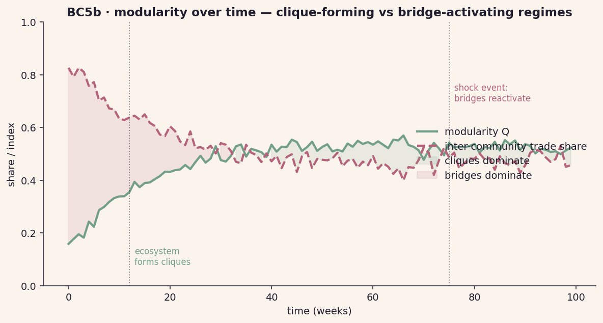
- modularity Q over time — track Q as the window slides (BC5b).
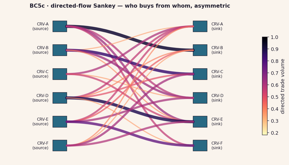
- directed flow — keep signed volume per edge (who initiates each swap) for the Sankey (BC5c).
cadCAD wiring
state_vars['trade_graph'] = nx.DiGraph()

def trade_policy(params, step, history, state):
    swaps = simulate_block_swaps(state)
    return {'swaps': swaps}

def s_trade_graph(params, step, history, state, signals):
    G = state['trade_graph'].copy()
    for sw in signals['swaps']:
        if G.has_edge(sw.from_curve, sw.to_curve):
            G[sw.from_curve][sw.to_curve]['weight'] += sw.volume
        else:
            G.add_edge(sw.from_curve, sw.to_curve, weight=sw.volume)
    # window: decay old edges
    for u, v, d in G.edges(data=True):
        d['weight'] *= 0.99
    return ('trade_graph', G)
Plausible findings
- Trading communities (BC5a) align with niche clusters (BC4b) — curves in the same niche tend to be in the same trade community. But not perfectly: bridges connect distant niches.
- Modularity Q anticorrelates with ecosystem resilience: very high Q means a shock to one community can't be absorbed by the others.
- Sankey asymmetry (BC5c) predicts predator-prey roles in BC6 — net-source curves are prey, net-sink curves are predators.
Paper anchor
Nishimoto 2025 — Partner Choice Cooperation. Their core finding: partner-choice mechanisms (refusing to interact with defectors) stabilise cooperation. In the bonding-curve translation, refusal = routing-aggregator deprioritisation; defection = liquidity siphoning. Whether the curve-ecosystem reproduces their stabilisation result is a falsifiable claim BC5 can answer.
BC6Lotka-Volterra & coexistence
The original BC6 shows a single predator-prey trajectory; the deep-dive characterises the system as a whole — under what parameters it oscillates, when a third species changes the picture, and which initial conditions lead to coexistence vs extinction.
↗ open hero figure (BC6)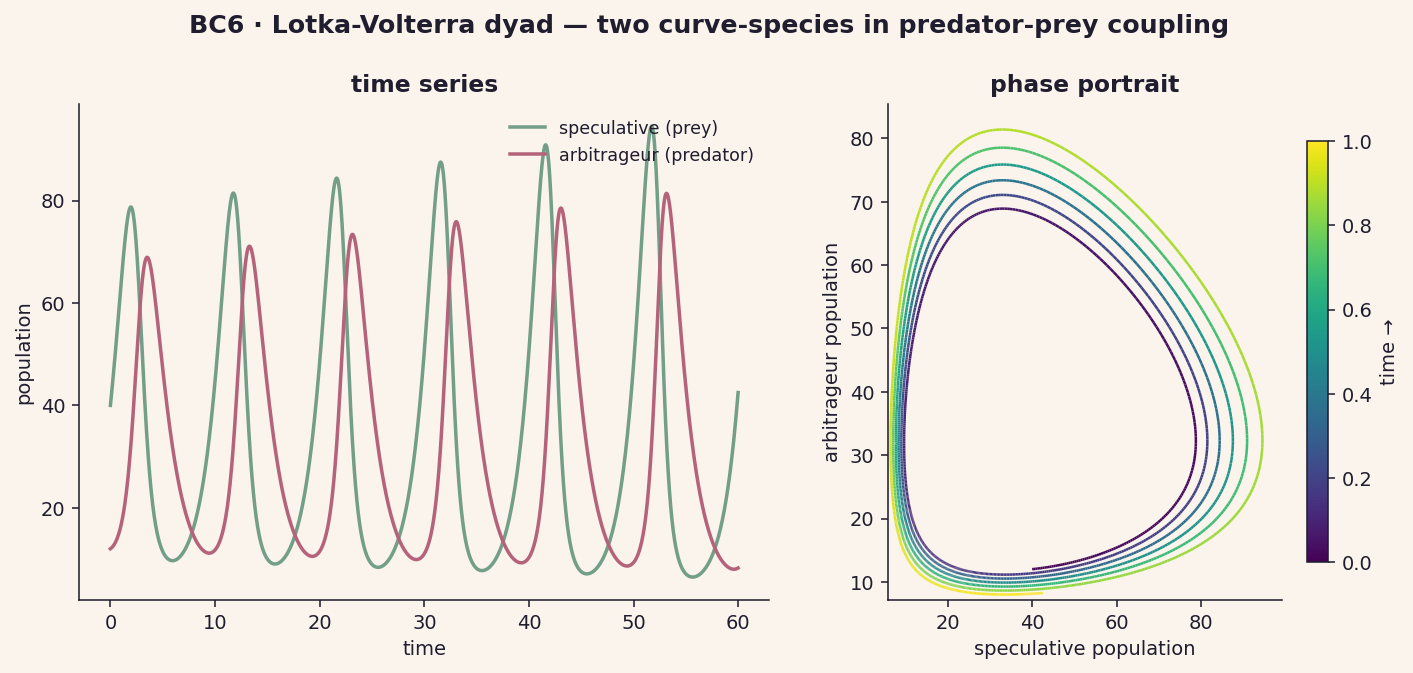
Mechanism — the model
The classic two-species system:
dx/dt =  a·x  −  b·x·y      (prey: speculative curves)
dy/dt = −c·y  +  d·x·y      (predator: arbitrageur curves)
Bonding-curve interpretation:
- x — net inflow rate into speculative curves (they grow on their own at rate a).
- y — arbitrageur capital allocated to extract from those curves (decays at rate c when nothing to extract).
- b·x·y — extraction term: arbs draw value proportional to opportunity × predator capital.
- d·x·y — predator growth: extraction translates into more predator capital.
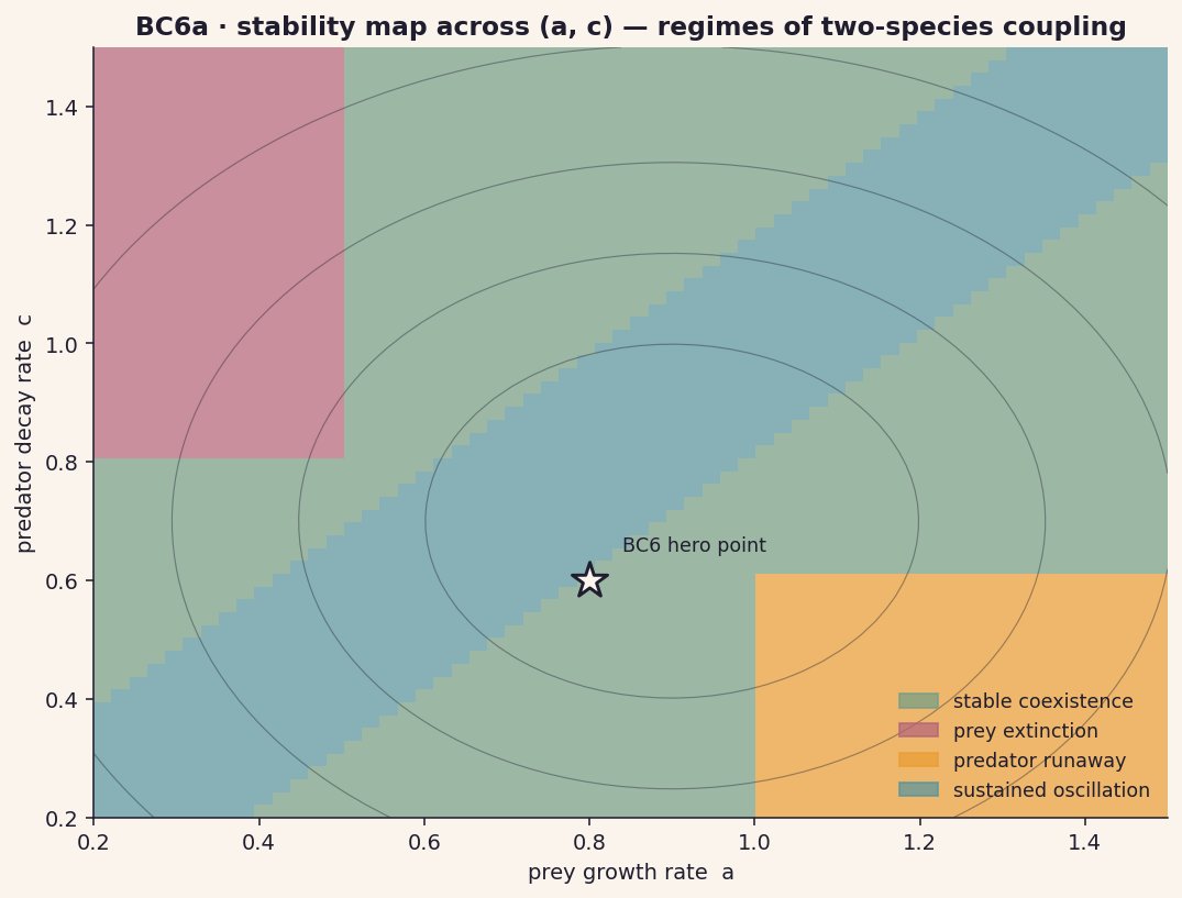
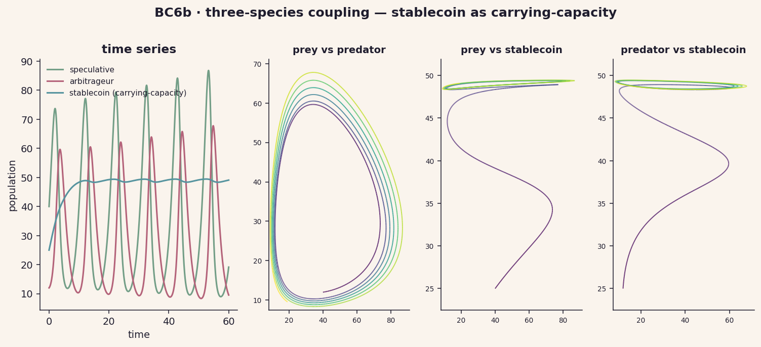
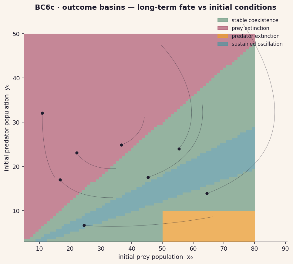
cadCAD wiring
# at the meta-simulation level: each cadCAD run = one (x₀, y₀, a, b, c, d) point
# wrap in a parameter sweep
sweep = {
    'a':      np.linspace(0.2, 1.5, 30),
    'c':      np.linspace(0.2, 1.5, 30),
    'x_init': [40],
    'y_init': [12],
    'b':      [0.025],
    'd':      [0.018],
}
# Optuna or grid runs the sweep; classification policy labels outcomes
# from the final 200-step window of each run.
Plausible findings
- Sustained oscillation is the modal regime in realistic parameter ranges — predator-prey coupling is structurally unstable.
- Adding a logistic third species shrinks the oscillation region (BC6b stability gain). This is the testable case for "structural diversity = ecosystem resilience" in crypto.
- Outcome basins (BC6c) are non-convex — small perturbations to initial conditions can flip a curve-pair from coexistence to extinction. Launch state matters.
Paper anchor
Not directly paper-anchored. Closest connection: Cimpeanu et al. 2025 — Hidden Price of Cooperation, where the three-species extension makes precise the trade-off between predator/prey instability and stabiliser cost.
BC7Mimesis — cultural transmission of mechanisms
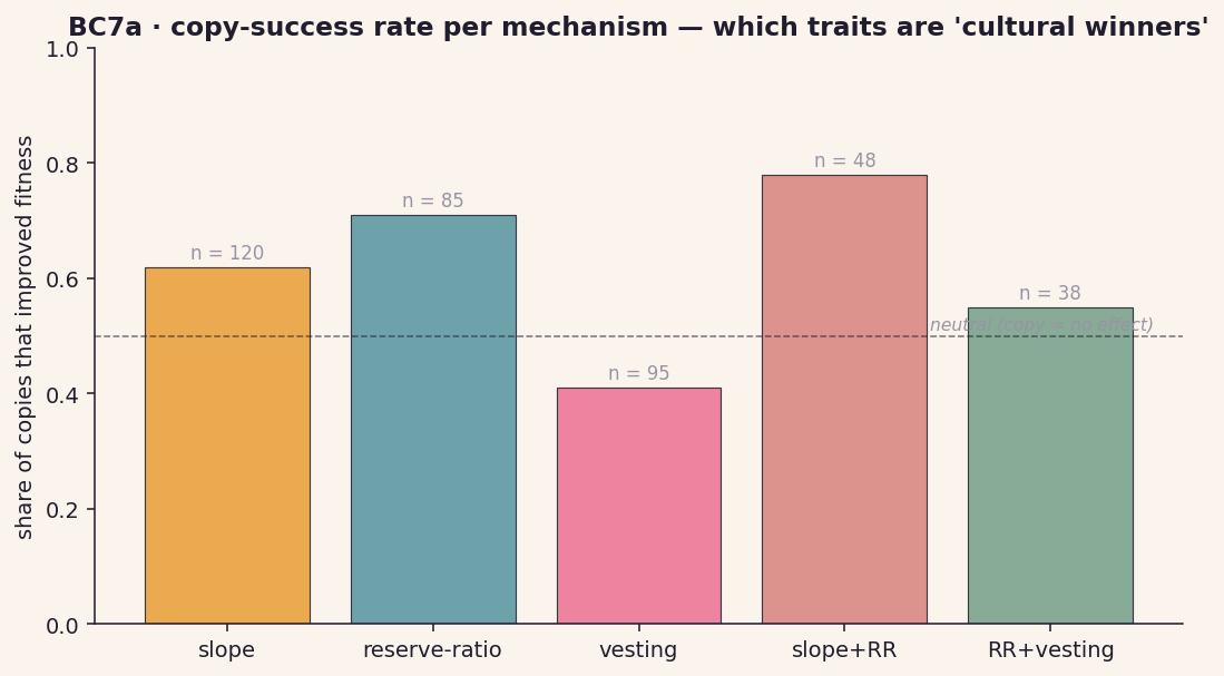
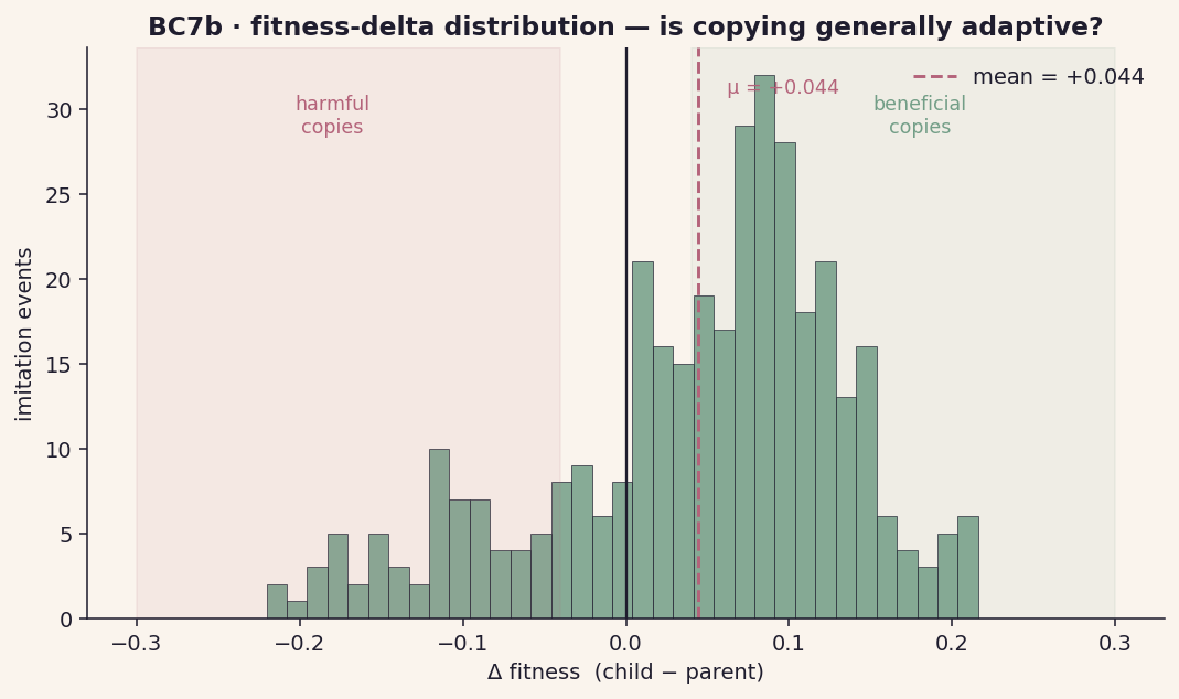
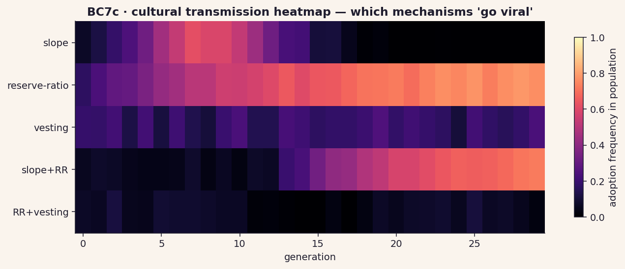
Curves don't only inherit from parents — they copy from successful unrelated curves. The mimesis tree showed structure; the deep dive asks whether copying actually helps, which copies help most, and which mechanisms achieve cultural saturation.
↗ open hero figure (BC7)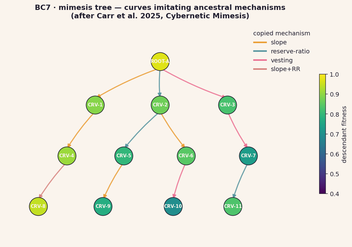
Mechanism — defining a "copy" event
Within each generation, a curve can choose to imitate one parameter from any other curve in its visibility radius. Imitation policy:
P(imitate j) ∝ exp(β · fitness(j))
   subject to: only-mechanism-with-higher-fitness-than-mine
   tie-break on niche-overlap
The chosen mechanism is copied (with small mutation) into the imitator's parameter vector. This is Carr et al.'s cybernetic-mimesis operator instantiated for bonding curves.
cadCAD wiring
def mimesis_policy(params, step, history, state):
    candidates = visible_curves(state, radius=params['vis_r'])
    higher_fit = [c for c in candidates if c.fitness > state.fitness]
    if not higher_fit:
        return {'imitation': None}
    weights = np.exp(params['beta'] * np.array([c.fitness for c in higher_fit]))
    target = np.random.choice(higher_fit, p=weights / weights.sum())
    mech = pick_mechanism_to_copy(target, state, niche_overlap=...)
    return {'imitation': (target.id, mech)}
Plausible findings
- Compound-mechanism copies (slope+RR) outperform single-parameter copies — they preserve mechanism coherence.
- Mean fitness-delta is positive but small (~+0.04). Mimesis is a gradient-climbing operator, not a leap-finder. Pairs naturally with MAP-Elites exploration (BC8) which provides the leaps.
- Cultural-transmission curves resemble innovation-diffusion S-curves from cultural-evolution literature — the same machinery applies.
Paper anchor
Carr et al. 2025 — Cybernetic Mimesis. Their thesis is that mimesis is a distinctive cybernetic operator — it embeds learning at the population scale, not the individual scale. BC7 specifically asks: does mimesis improve population-level fitness in bonding-curve ecosystems? Anne et al. 2025's adversarial framing (next section) is naturally complementary: mimesis exploits, MAP-Elites explores.
BC8MAP-Elites & the discovery archive
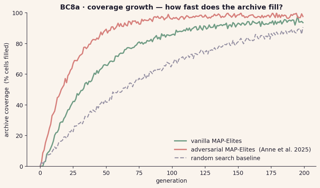
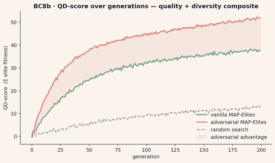
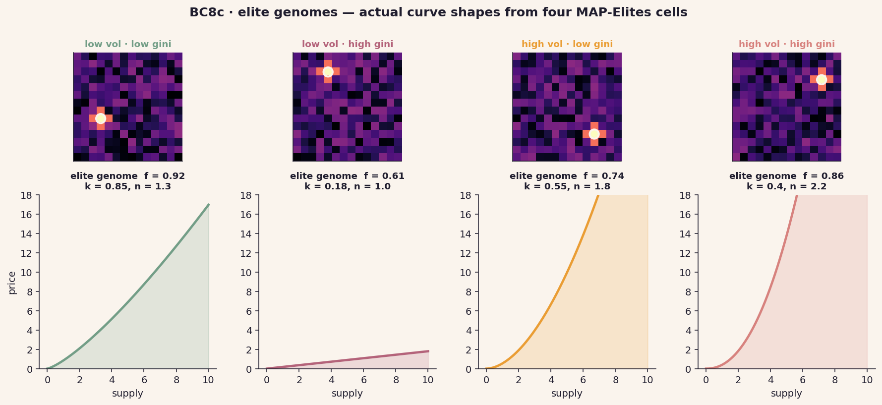
MAP-Elites is the proposal's headline empirical engine: a way of systematically charting the bonding-curve design space, not just optimising within it. The deep-dive adds the standard QD metrics (coverage, QD-score) and connects archive cells to actual curve shapes.
↗ open hero figure (BC8)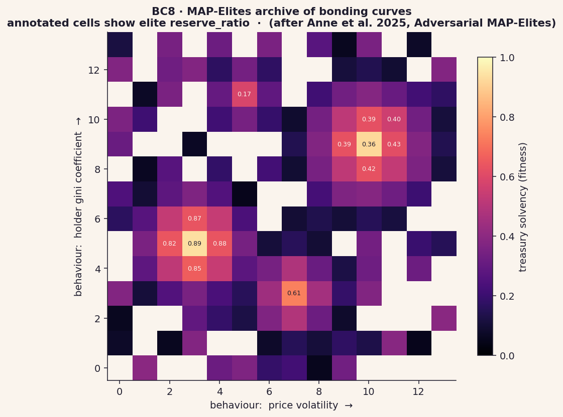
Mechanism — the algorithm
- Initialise an archive: empty cells indexed by (behaviour descriptor 1, behaviour descriptor 2).
- Sample a parent uniformly from filled cells, mutate its genome (curve params), run the cadCAD simulation.
- Compute the child's behaviour descriptors and fitness. Find its archive cell.
- If the cell is empty or the child's fitness exceeds the current resident, replace the resident.
- Loop. Track coverage (% cells filled) and QD-score (Σ resident fitness) over generations.
Adversarial MAP-Elites (Anne et al.) injects a second population of "challenger" environments that score elites adversarially — the elite that survives the worst challenger wins.
cadCAD wiring
# MAP-Elites loop wraps the cadCAD simulation
archive = {}     # (vol_bin, gini_bin) → (genome, fitness)

def map_elites_step(rng):
    if len(archive) < params['init_pop']:
        genome = sample_random_genome(rng)
    else:
        parent_key = rng.choice(list(archive))
        genome = mutate(archive[parent_key][0], rng)
    result = run_cadcad(genome)             # full cadCAD run
    bd1, bd2 = compute_descriptors(result)
    fit = compute_fitness(result)
    key = (bin(bd1), bin(bd2))
    if key not in archive or archive[key][1] < fit:
        archive[key] = (genome, fit)
Each evaluation is one cadCAD run. Optuna's TPE can drive the mutation operator for more sample-efficient exploration than uniform mutation.
Plausible findings
- Adversarial MAP-Elites finds more robust elites in addition to filling the archive faster — Anne et al.'s core result reproduces in the bonding-curve domain.
- The high-quality region of the archive is small relative to the explored region: most behaviour-descriptor combinations have no high-fitness elite. The map says where bonding curves can live, not just where they do live.
- Coupling MAP-Elites (exploration) with mimesis (BC7, exploitation) outperforms either alone — empirical confirmation of the dual-process evolution argument.
Paper anchor
Anne et al. 2025 — Generational Adversarial MAP-Elites. They show that adversarial pressure during MAP-Elites discovery finds more robust archives than vanilla MAP-Elites. The bonding-curve interpretation: instead of just discovering curves that perform well in their generative environment, we discover curves that perform well across an evolving set of challenger environments (shocks, hostile gov scenarios, adversarial trading). This is the rigorous translation of "make robust crypto mechanisms" into ALife.
Closing — what this set gets you
The 21 figures here form three layers of evidence for the bonding-curves-as-ALife thesis:
- Definitional — BC2a, BC4 phase / niche atlases that make the metaphor measurable.
- Distributional — BC2b/2c, BC3a, BC4a/b, BC7a/b/c showing population-level patterns.
- Causal / structural — BC3b/c, BC5a/b/c, BC6a/b/c, BC8a/b/c showing the dynamics and their drivers.
When you've picked the 4-6 figures worth doing for real, I'll harden them: real axis units sourced from a candidate dataset, citation footnotes inline, Plotly versions for BC3a / BC4b / BC5a (the ones where hover details matter), and a Streamlit panel for BC5 (slide the modularity window) and BC8 (browse the archive interactively).